What VSWR Is Really Telling You: A Guide to Reflected Power and Impedance Uniformity

Key Takeaways

• VSWR is not just a pass/fail number. It is a diagnostic that reflects the impedance uniformity of the cable, the quality of the connector termination, and the compensation designed into the connector interface.
• An ideal VSWR of 1.0:1 is the theoretical target; practical systems must define an acceptable maximum and design to stay within it across the full operating frequency range.
• Reflections are additive. Multiple small impedance discontinuities across the cable and connector can combine to produce a significantly elevated VSWR.
• The connector is often the highest-risk point in the RF path; it must maintain 360-degree electrical contact and compensate for the geometric transition at the interface.
• Physical integrity directly affects electrical performance. Mechanical damage to a cable’s geometry will always appear in the VSWR measurement.

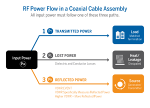
Imagine having a conversation in a long tunnel. You speak clearly, but somewhere down the tunnel a wall has been built; not completely solid, but enough to bounce your voice back toward you. The result is an echo that muddles the original message. This is a reasonable analogy for what happens when RF energy travels down a coaxial cable and encounters an impedance discontinuity. The reflected energy doesn’t disappear, it travels back toward the source, corrupting your signal and wasting transmit power. That reflection is exactly what Voltage Standing Wave Ratio (VSWR) measures.

VSWR is one of the most cited figures of merit in RF engineering, but it is frequently treated as nothing more than a pass-or-fail number. In reality, it is a diagnostic window into the physical and electrical integrity of the entire transmission path: the cable itself, the connectors, and every transition in between. Understanding what drives it, and how it relates to the uniformity of the cable’s internal geometry, is foundational to making good cable selection decisions.

What Is VSWR?

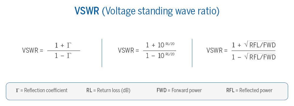
Voltage Standing Wave Ratio is a measurement of reflected voltage. Specifically, it quantifies the difference between the actual input impedance of a transmission line at any given point and the average characteristic impedance the system was designed around. It is expressed as a ratio, where 1.0:1 is the ideal: no reflection, all power delivered to the load.

That ratio climbing above 1.0:1 is an indication that energy is being reflected back toward the source. A VSWR of 2.0:1, for example, means roughly 11% of your input power is reflected rather than delivered. At 3.0:1, that rises to 25%. In precision systems, such as radar, satellite communications, and test and measurement equipment, even modest reflected power can be the difference between a system that works and one that doesn’t.

What VSWR Is Actually Judging

Low VSWR is used as a figure of merit for coaxial components because it indicates three distinct factors simultaneously:

• How well the physical uniformity of the cable is maintained along its entire length. Any variation in the geometry of the inner conductor, dielectric, or outer conductor creates a local impedance deviation that causes reflection. 

• Whether the connectors are properly designed and correctly attached; a connector that doesn’t make clean, uniform contact with the cable’s outer conductor introduces a discontinuity at the most critical junction. 
• How well the transitions between line sizes are compensated for in the connectors. Wherever the RF path changes diameter, compensation must be built into the connector design to maintain electrical continuity. 

Impedance Uniformity: The Physical Root of VSWR

Characteristic impedance in a coaxial cable is set by the ratio of the outer conductor’s inner diameter to the center conductor’s outer diameter, modulated by the dielectric constant of the insulating material between them. The formula is elegant, but the manufacturing reality is that maintaining perfectly uniform geometry along the full length of a cable, especially a flexible one, is a genuine challenge.

Any deviation from that ideal geometry, however small, creates a localized impedance change. The energy traveling down the cable “sees” a change in the medium it’s propagating through and partially reflects. These reflections are additive; multiple small discontinuities across the cable’s length can combine to produce a VSWR measurement that is far worse than any individual deviation would suggest on its own.

This is why VSWR is such a powerful diagnostic tool. It integrates the effect of every physical imperfection in the transmission path into a single measurable ratio. If VSWR is high, something in the geometry is wrong, and that something may be in the cable construction, the connector termination, or both.

The Connection Between VSWR and Signal Loss

VSWR and attenuation are related, but they measure different phenomena. VSWR captures reflected energy (mismatched loss); attenuation captures the energy that is absorbed or dissipated before it reaches the load. Both erode your link budget, but through different mechanisms, and the two effects compound each other.

A cable with marginal VSWR is already losing power to reflection; if that same cable has elevated attenuation, the signal arriving at the load is a double casualty.

Why the Connector Is the Most Vulnerable Point

A well-manufactured cable can have excellent impedance uniformity along its run length, only to have that performance destroyed by a poorly terminated or mismatched connector. The connector interface is where the RF energy must transition from the cable’s internal geometry to the mating interface of the system, and that transition must be managed carefully.

Connectors must maintain 360-degree contact with the cable’s outer conductor at the termination point. Any gap or inconsistency in that contact breaks the electrical continuity of the shield and creates a reflection point. The connector body must also be designed to compensate for the change in geometry that occurs as the coaxial structure transitions to the mating interface. This is why the same cable terminated with two different connector designs, or even two different termination techniques, can produce noticeably different VSWR results.

Structural Return Loss: Another Way to See the Same Problem

Impedance dis-uniformities, which are the result of the cable manufacturing process, are what is referred to as Structural Return Loss. Potential dis-uniformities may result from improper control of the many variables involved in the process. However, most often when we’re referring to Structural Return Loss with a coaxial cable, it’s the result of periodic flaws built into the cable during manufacturing. These flaws can be microscopic but will show themselves as narrow band reflections (spikes) at a frequency having a quarter wavelength equivalent to the distance between these periodic flaws. The magnitude of these potential spikes will increase when measuring a longer length of cable. Common causes can be poorly maintained gear boxes, bearings, cams, or other similar components.

A structural return loss spike will result in a corresponding suck-out of attenuation at that same frequency. The impact to a system could be significant if the operating frequency of a system is located very close to one of these spikes.

Semi-Rigid Performance with Greater Flexibility

Semi-rigid cable maintains highly uniform impedance through the consistent geometry of its smooth center conductor, dielectric, and solid outer conductor, but its rigid construction can make routing and installation more difficult. MilTech® and MaxGain® cable assemblies are designed to mimic the construction and electrical performance of semi-rigid cable while providing greater flexibility. This helps maintain impedance uniformity and reliable VSWR performance in applications where traditional semi-rigid cable may be difficult to install.

The Interplay with Shielding and Mechanical Integrity

The outer conductor of a coaxial cable is doing two things simultaneously: it defines the outer boundary of the impedance-controlling geometry, and it acts as the electromagnetic shield that keeps the signal isolated from the outside world. Any physical distortion, such as kink, a crush point, or an uneven braid tension, changes that geometry and degrades VSWR. These two functions cannot be separated, which is why shielding construction choices and impedance uniformity are deeply intertwined.

And that mechanical integrity conversation goes further than the cable itself. Every bend, every clamp, every connector torquing event physically changes the geometry that VSWR is measuring. An over-bent cable or one that has been crushed under a cable clamp will show VSWR degradation that no amount of connector improvement can fix.

FAQ

What is a good VSWR for a coaxial cable?

A VSWR of 1.0:1 is the theoretical ideal, indicating zero reflected power. In practice, system requirements define the acceptable maximum. Many precision RF applications specify 1.25:1 or better across the operating frequency range. What matters is maintaining that specification at the highest operating frequency, where reflections are most significant.

What causes high VSWR in a cable assembly?

High VSWR is almost always the result of a physical geometry problem somewhere in the RF path. The most common causes are impedance discontinuities in the cable itself (from manufacturing variation, mechanical damage, or over-bending), poorly terminated connectors that don’t maintain 360-degree contact with the outer conductor, or uncompensated line-size transitions within the connector body.

Is VSWR the same as return loss?

They measure the same phenomenon, reflected power, but express it differently. Return loss is expressed in decibels (dB) and uses a negative scale where a larger number means better performance. VSWR is expressed as a ratio (e.g., 1.5:1) and is often more intuitive for comparing cable and connector specs. The two are mathematically interconvertible.

Does VSWR change with frequency?

Yes, VSWR generally increases with frequency for a given cable and connector, which is why specifications are evaluated across the full operating frequency range rather than at a single point. A cable that passes at 1 GHz may fail at 18 GHz if connector compensation or cable geometry uniformity isn’t maintained across the band.